Objectives
In our first set of labs we will be getting familiar with Microsoft Excel, a tool used by many organisations to evaluate daily performance and to make critical strategic and operational decisions.
This first lab will briefly review some of the fundamental skills needed to use Excel. This is not meant to be a complete tutorial; many good Excel tutorials can be found online.
Using Microsoft Excel
Spreadsheet software for personal computers has become an indispensable tool for business analysis, particularly for the manipulation of numberical data and the development and analysis of decision models. Some differences exist between 2007 and 2010. If you do use another version you should be able to apply Excel easily to the problems and exercises. In addition it must be noted that Mac versions of Excel do not have the full funcitonality that Windows versions have.
Although Excel has some flaws and limitations from a statistical perspective, its widespread availability makes it the software of choice for many business professionals.
Instructions for working in Walton Building PC Labs:
If you are working on the workstations in the IT Building all machines should be installed with Microsoft Excel 2010.
Proceed with the next step of the lab.
Instructions for working on your own laptop
You must have a copy of Microsoft Excel 2010 or newer installed.
There will be adons utilised in future practicals but for the moment the standard installation of Excel is sufficient. The student site that supports a book used in this module contains the links to software, along with data files and other materials.
The Basics
This lab assumes you are familiar with the most elementary spreasheet concepts and procedures:
- Opening, saving and printing files.
- Moving around a spreadsheet.
- Selecting ranges.
- Inserting/deleting rows and columns
- Entering and editing text, numerical data, and formulas.
- Formating data.
- Working with text strings.
- Performing basic arithmetic calculations.
- Modifying the appearance of the spreadsheet.
- Sorting data.
File to use
Download the following file and open it in Excel
Copying Formulas
Excel provides several ways of copying formulas to different cells. This is extremely useful in building decision models, because many models require replication of formulas for different periods of time, similar products, and so on.
One way is to select the cell with the formula to be copied, click the copy button from the clipboard group on the ribbon (or click Ctrl+C), click on the cell you wish to copy to and click the paste button (or click Ctrl+V).
You can also enter a formula into a range of cells by selecting the range of cells typing in the formula and press Ctrl+Enter. Use the small black square on a selected cell to copy the formula down a column or across a row.
The structure of the formula is the same as in the original cell but the cell references have been changed to reflect the relative addresses of the formula in the new cells.
Practice this using the science engineering data file. Calculate the difference between the jobs in each category from 2000 to 2010. To see all of your formulas on a worksheet you can use the Ctrl+` keys to toggle viewing and hiding formulas.
Sometimes when you copy a formula you do not want the cell references to change. For example, calculate the percent of the total jobs for each occupation in 2010. In cell E4 enter the formula =C4/$C$12. Then if you copy this formula down column E for the other occupations the numerator will change to reference each occupation but the denominator will still point to cell C12. You should be careful to use relative and absolute addressing appropriately in your models. To convert a relative reference to an absolute one, just press F4 when you are in the cell reference.
Order of Arithmetic
Excel uses standard "PEMDAS" order of operations for arithmetic. Parenthese, Exponents, Multiplication and Division, Addition and Subtraction.
    Parentheses    (6-1)
    Exponents ^
    Multiplication *
    Division /
    Addition +
    Subtraction -


    Assume we want (6-3)(4+2) = 18
    In Excel we write =(6-3)*(4+2)

    Assume we want (3/5) squared
    In Excel we write =(3/5)^2
Formulas
To see formula's in a cell you can precede the formula with a apostrophe, then excel will not activate the formula until you remove the apostrophe.
Functions
The functions available in Excel beyond arithmetic are extensive. There are hundreds of built in functions. Some functions are those that work within a cell and some work on sets of cells.
Individual Cell Functions:
Functions are used to perform functions on individual cells.
- ln(number) natural log
- log(number,base) log to the base
- pi()
- rand() random number generator
Groups of cells (Array) functions
Functions are used to perform special calculations in groups of cells. Some of these more common functions used in statistical applications include:
- MIN(range)
- MAX(range)
- SUM(range)
- AVERAGE(range)
- COUNT(range)
- COUNTIF(range,criteria)
- AND(condition1, condition2...) returns true if all conditions are true and false if not.
- OR(condition1, condition2...) returns ture is any condition is true and false if not.
- IF(condition, value if true, value if false) returns one value if the condition is true and another if it is false.
- VLOOKUP(value, table range, column number) looks up a value in a table.
The easiest way to locate a particular funciton is to select a cell and click on the Insert function button on the ribbon. This is useful when you know the name of the function but are unsure of the arguments.
Using the science and egineering data include some formulas to find the maximum, minimum, and total for the number of jobs difference. What is the average difference?
Functions on a set of numbers
The natural log of a number is used in business to figure out growth rates over time. ln(x) is the natural log of number x. The natural log of 1.5:
- Assuming 100% growth rate you are essentially asking how long does it take to grow to get to 1.5, the answer is .405, less than half the time period)
- Assuming 1 period of time, how much do you need to grow to get to 1.5 (40.5% per year)
You are either looking at growth rate or time period.
Save the following stock prices file.
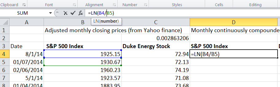
We can perform functions on more than one variable such as pairs, two rows or two columns perhaps. This data is from Yahoo finance for the Standard and Poor's 500 index (US stock market index) and Duke Energy stock prices. The price is the closing price from the begining of each month. 176 months of price data. We want to caculate the continuously commounded monthly return. To do this we take the natural log of the ratio between the two prices with the more recent price on top.
We do the natural log function of the price in August, divided by the price in July, this gives us a loss of -.29% In August the index was 1925.15 and in July it was 1930.67
This applies the natural log function to show the monthly continuously compounded return.
Now double click on the handle of cell D4 so that the remainder of the cell in column D are populated. Then copy the formula to cell E4 and populate all column E.
Duke Energy prices show as slightly up for the month 1.12%.
This shows two time series of monthly returns for the index and for an idividual stock. You may now want to see how one stock performed agains the larger market it is a part of. Which performed better?
To calcualte the average of a series of values that are all in one column or one row (an array), we write a formula into cell G6
=Average(D4:D178).Then copy that relative reference formula over to cell H6
To find the average annual return in cell G8 then we multiply by 12. Again copy this formula over to H8.
Calculate the standard deviation of monthly returns in cell G10 using the stdev.p() function.
To calcuate the annualised standard deviation we do not simply multiply by 12 we must multiple by the squareroot of 12. Excel has a function for this so in cell G12 enter the following:
=G10*sqrt(12)Now calculate the minimum and maximum for both the index and for Duke Energy stock.
We can see from the descriptive statistics that conclusions can be made; Duke Energy Stock has been much higher paying investment that investing in S&P over this time ineterval (14 years), there was a higher standard deviation of returns so Duke is not a free deal it has some cost in terms of risks.
Excel charts
Raw data is often hard to interpret, charts and graphs provide a convenient way to visualise data and provide information and insight for making better decisions. Excel provides vertical and horizontal bar charts, line charts, pie charts, area charts, scatter plots, three-dimensional charts and many others.
Column and Bar charts
Excel calls vertical bar charts, column charts and horizontal bar charts, bar charts.
Open the file:
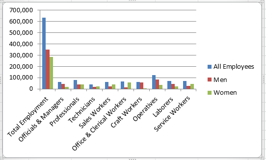
Create a column chart for the EEO Employment Report data.
Use the data for All employees, Men and Women, (rows 4,5 and 6) the chart should show the number of workers in each category.
What does a stacked chart look like?
Line charts
Line charts provide a useful means for displaying data over time. You can plot multiple data series in line charts; however, they can be difficult to interpret if the magnitude of the data values differs greatly. Create a line chart for the closing prices in the Excel file SP500
We will cover charts more extensively in week 6.
More Charts
- Experiment with the other charts that are available.
- Line charts provide a useful means for displaying data over time.
- Create a line chart for the closing prices in the file SP500.xlsx
- For many types of data, we are interested in understanding the relative proportion of each data source to the total.
- Create a pie chart showing the breakdown of occupations in the Science-engineering.xlsx